Vector data in Python

Overview

Teaching: 30 min
Exercises: 20 min

Questions

• How can I distinguish between and visualize point, line and polygon vector data?

Objectives

• Know the difference between point, line, and polygon vector elements.

• Load point, line, and polygon vector data with geopandas.

• Access the attributes of a spatial object with geopandas.

Introduction

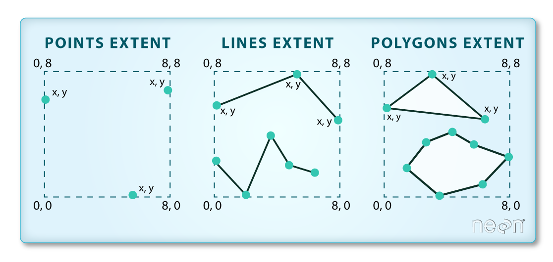
As discussed in Episode 2: Introduction to Vector Data, vector data represents specific features on the Earth’s surface using points, lines and polygons. These geographic elements can then have one or more attributes assigned to them, such as ‘name’ and ‘population’ for a city, or crop type for a field. Vector data can be much smaller in (file) size than raster data, while being very rich in terms of the information captured.

In this episode, we will be moving from working with raster data to working with vector data. We will use Python to open and plot point, line and polygon vector data. In particular, we will make use of the geopandas package to open, manipulate and write vector datasets. geopandas extends the popular pandas library for data analysis to geospatial applications. The main pandas objects (the Series and the DataFrame) are expanded by including geometric types, represented in Python using the shapely library, and by providing dedicated methods for spatial operations (union, intersection, etc.).

Introduce the Vector Data

The data we will use comes from the Dutch government’s open geodata sets, obtained from the PDOK platform. It provides open data for various applications, e.g. real estate, infrastructure, agriculture, etc. In this episode we will use three data sets:

• Crop fields (polygons)
• Water ways (lines)
• Ground water monitoring wells (points)

In later episodes, we will learn how to work with raster and vector data together and combine them into a single plot.

Import Vector Datasets

import geopandas as gpd

We will use the geopandas module to load the crop field vector data we downloaded at: data/brpgewaspercelen_definitief_2020_small.gpkg. This file contains data for the entirety of the European portion of the Netherlands, resulting in a very large number of crop field parcels. Directly loading the whole file to memory can be slow. Let’s consider as Area of Interest (AoI) northern Amsterdam, which is a small portion of the Netherlands. We only need to load this part.

We define a bounding box, and will only read the data within the extent of the bounding box.

# Define bounding box
xmin, xmax = (110_000, 140_000)
ymin, ymax = (470_000, 510_000)
bbox = (xmin, ymin, xmax, ymax)

How should I define my bounding box?

For simplicity, here we assume the Coordinate Reference System (CRS) and extent of the vector file are known (for instance they are provided in the dataset documentation). Some Python tools, e.g. fiona(which is also the backend of geopandas), provides the file inspection functionality without actually the need to read the full data set into memory. An example can be found in the documentation of fiona.

Using the bbox input argument, we can load only the spatial features intersecting the provided bounding box.

# Partially load data within the bounding box
cropfield = gpd.read_file("data/brpgewaspercelen_definitief_2020_small.gpkg", bbox=bbox)

Vector Metadata & Attributes

When we import the vector dataset to Python (as our cropfield object) it comes in as a DataFrame, specifically a GeoDataFrame. The read_file() function also automatically stores geospatial information about the data. We are particularly interested in describing the format, CRS, extent, and other components of the vector data, and the attributes which describe properties associated with each individual vector object.

Spatial Metadata

Key metadata includes:

1. Object Type: the class of the imported object.
2. Coordinate Reference System (CRS): the projection of the data.
3. Extent: the spatial extent (i.e. geographic area that the data covers). Note that the spatial extent for a vector dataset represents the combined extent for all spatial objects in the dataset.

Each GeoDataFrame has a "geometry" column that contains geometries. In the case of our cropfield object, this geometry is represented by a shapely.geometry.Polygon object. geopandas uses the shapely library to represent polygons, lines, and points, so the types are inherited from shapely.

We can view the metadata using the .crs, .bounds and .type attributes. First, let’s view the geometry type for our crop field dataset. To view the geometry type, we use the pandas method .type on the GeoDataFrame object, cropfield.

cropfield.type

0        Polygon
1        Polygon
2        Polygon
3        Polygon
4        Polygon
          ...
22026    Polygon
22027    Polygon
22028    Polygon
22029    Polygon
22030    Polygon
Length: 22031, dtype: object

To view the CRS metadata:

cropfield.crs

<Derived Projected CRS: EPSG:28992>
Name: Amersfoort / RD New
Axis Info [cartesian]:
- X[east]: Easting (metre)
- Y[north]: Northing (metre)
Area of Use:
- name: Netherlands - onshore, including Waddenzee, Dutch Wadden Islands and 12-mile offshore coastal zone.
- bounds: (3.2, 50.75, 7.22, 53.7)
Coordinate Operation:
- name: RD New
- method: Oblique Stereographic
Datum: Amersfoort
- Ellipsoid: Bessel 1841
- Prime Meridian: Greenwich

Our data is in the CRS RD New. The CRS is critical to interpreting the object’s extent values as it specifies units. To find the extent of our dataset in the projected coordinates, we can use the .total_bounds attribute:

cropfield.total_bounds

array([109222.03325 , 469461.512625, 140295.122125, 510939.997875])

This array contains, in order, the values for minx, miny, maxx and maxy, for the overall dataset. The spatial extent of a GeoDataFrame represents the geographic “edge” or location that is the furthest north, south, east, and west. Thus, it is represents the overall geographic coverage of the spatial object. Image Source: National Ecological Observatory Network (NEON).

We can convert these coordinates to a bounding box or acquire the index of the dataframe to access the geometry. Either of these polygons can be used to clip rasters (more on that later).

Selecting spatial features

Sometimes, the loaded data can still be too large. We can cut it is to a even smaller extent using the .cx indexer (note the use of square brackets instead of round brackets, which are used instead with functions and methods):

# Define a Boundingbox in RD
xmin, xmax = (120_000, 135_000)
ymin, ymax = (485_000, 500_000)
cropfield_crop = cropfield.cx[xmin:xmax, ymin:ymax]

This will cut out a smaller area, defined by a box in units of the projection, discarding the rest of the data. The resultant GeoDataframe, which includes all the features intersecting the box, is found in the cropfield_crop object. Note that the edge elements are not ‘cropped’ themselves. We can check the total bounds of this new data as before:

cropfield_crop.total_bounds

array([119594.384, 484949.292625, 135375.77025, 500782.531])

We can then save this cropped dataset for use in future, using the to_file() method of our GeoDataFrame object:

cropfield_crop.to_file('cropped_field.shp')

This will write it to disk (in this case, in ‘shapefile’ format), containing only the data from our cropped area. It can be read in again at a later time using the read_file() method we have been using above. Note that this actually writes multiple files to disk (cropped_field.cpg, cropped_field.dbf, cropped_field.prj, cropped_field.shp, cropped_field.shx). All these files should ideally be present in order to re-read the dataset later, although only the .shp, .shx, and .dbf files are mandatory (see the Introduction to Vector Data lesson for more information.

Plotting a vector dataset

We can now plot this data. Any GeoDataFrame can be plotted in CRS units to view the shape of the object with .plot().

cropfield_crop.plot()

We can customize our boundary plot by setting the figsize, edgecolor, and color. Making some polygons transparent will come in handy when we need to add multiple spatial datasets to a single plot.

cropfield_crop.plot(figsize=(5,5), edgecolor="purple", facecolor="None")

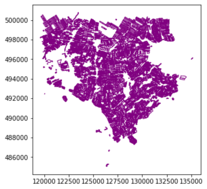
Under the hood, geopandas is using matplotlib to generate this plot. In the next episode we will see how we can add DataArrays and other vector datasets to this plot to start building an informative map of our area of interest.

Spatial Data Attributes

We introduced the idea of spatial data attributes in an earlier lesson. Now we will explore how to use spatial data attributes stored in our data to plot different features.

Challenge: Import Line and Point Vector Datasets

Using the steps above, load the waterways and groundwater well vector datasets (data/status_vaarweg.zip and data/brogmwvolledigeset.zip, respectively) into Python using geopandas. Name your variables waterways_nl and wells_nl respectively.

Answer the following questions:

1. What type of spatial features (points, lines, polygons) are present in each dataset?

2. What is the CRS and total extent (bounds) of each dataset?

3. How many spatial features are present in each file?

Answers

First we import the datasets:

waterways_nl = gpd.read_file("data/status_vaarweg.zip")
wells_nl = gpd.read_file("data/brogmwvolledigeset.zip")

Then we check the types:

waterways_nl.type

wells_nl.type

We also check the CRS and extent of each object:

print(waterways_nl.crs)
print(waterways_nl.total_bounds)
print(wells_nl.crs)
print(wells_nl.total_bounds)

To see the number of features in each file, we can print the dataset objects in a Jupyter notebook or use the len() function. waterways_nl contains 91 lines and wells_nl contains 51664 points.

Challenge: Investigate the waterway lines

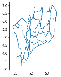
Now we will take a deeper look in the Dutch waterway lines: waterways_nl. Let’s visualize it with the plot function. Can you tell what is wrong with this vector file?

Answers

By plotting out the vector file, we can tell that the latitude and longitude of the file are flipped.

waterways_nl.plot()

Axis ordering

According to the standards, the axis ordering for a CRS should follow the definition provided by the competent authority. For the commonly used EPSG:4326 geographic coordinate system, the EPSG defines the ordering as first latitude then longitude. However, in the GIS world, it is custom to work with coordinate tuples where the first component is aligned with the east/west direction and the second component is aligned with the north/south direction. Multiple software packages thus implement this convention also when dealing with EPSG:4326. As a result, one can encounter vector files that implement either convention - keep this in mind and always check your datasets!

Modify the geometry of a GeoDataFrame

Sometimes we need to modify the geometry of a GeoDataFrame. For example, as we have seen in the previous exercise Investigate the waterway lines, the latitude and longitude are flipped in the vector data waterways_nl. This error needs to be fixed before performing further analysis.

Let’s first take a look on what makes up the geometry column of waterways_nl:

waterways_nl['geometry']

0     LINESTRING (52.41810 4.84060, 52.42070 4.84090...
1     LINESTRING (52.11910 4.67450, 52.11930 4.67340...
2     LINESTRING (52.10090 4.25730, 52.10390 4.25530...
3     LINESTRING (53.47250 6.84550, 53.47740 6.83840...
4     LINESTRING (52.32270 5.14300, 52.32100 5.14640...
                            ...
86    LINESTRING (51.49270 5.39100, 51.48050 5.39160...
87    LINESTRING (52.15900 5.38510, 52.16010 5.38340...
88    LINESTRING (51.97340 4.12420, 51.97110 4.12220...
89    LINESTRING (52.11910 4.67450, 52.11850 4.67430...
90    LINESTRING (51.88940 4.61900, 51.89040 4.61350...
Name: geometry, Length: 91, dtype: geometry

Each row is a LINESTRING object. We can further zoom into one of the rows, for example, the third row:

print(waterways_nl['geometry'][2])
print(type(waterways_nl['geometry'][2]))

LINESTRING (52.100900002 4.25730000099998, 52.1039 4.25529999999998, 52.111299999 4.24929999900002, 52.1274 4.23449999799999)
<class 'shapely.geometry.linestring.LineString'>

As we can see in the output, the LINESTRING object contains a list of coordinates of the vertices. In our situation, we would like to find a way to flip the x and y of every coordinates set. A good way to look for the solution is to use the documentation of the shapely package, since we are seeking to modify the LINESTRING object. Here we are going to use the shapely.ops.transform function, which applies a self-defined function to all coordinates of a geometry.

import shapely

# Define a function flipping the x and y coordinate values
def flip(geometry):
    return shapely.ops.transform(lambda x, y: (y, x), geometry)

# Apply this function to all coordinates and all lines
geom_corrected = waterways_nl['geometry'].apply(flip)

Then we can update the geometry column with the corrected geometry geom_corrected, and visualize it to check:

# Update geometry
waterways_nl['geometry'] = geom_corrected

# Visualization
waterways_nl.plot()

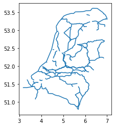
Now the waterways look good! We can save the vector data for later usage:

# Update geometry
waterways_nl.to_file('waterways_nl_corrected.shp')

Key Points

• Vector dataset metadata include geometry type, CRS, and extent.

• Load spatial objects into Python with geopandas.read_file() function.

• Spatial objects can be plotted directly with GeoDataFrame’s .plot() method.