Crop raster data with rioxarray and geopandas

Overview

Teaching: 40 min
Exercises: 20 min

Questions

• How can I crop my raster data to the area of interest?

Objectives

• Crop raster data with a bounding box.

• Crop raster data with a polygon.

• Crop raster data within a geometry buffer.

It is quite common that the raster data you have in hand is too large to process, or not all the pixels are relevant to your area of interest (AoI). In both situations, you should consider cropping your raster data before performing data analysis.

In this episode, we will introduce how to crop raster data into the desired area. We will use one Sentinel-2 image over Amsterdam as the example raster data, and introduce how to crop your data to different types of AoIs.

Introduce the Data

We’ll continue from the results of the satellite image search that we have carried out in an exercise from a previous episode. We will load data starting from the search.json file.

If you would like to work with the data for this lesson without downloading data on-the-fly, you can download the raster data using this link. Save the geospatial-python-raster-dataset.tar.gz file in your current working directory, and extract the archive file by double-clicking on it or by running the following command in your terminal tar -zxvf geospatial-python-raster-dataset.tar.gz. Use the file geospatial-python-raster-dataset/search.json (instead of search.json) to get started with this lesson.

We also use the vector data that has already been introduced in episode Vector data in python.

Crop raster data with a bounding box

We load a true color image using pystac and rioxarray and check the shape of the raster:

import pystac
import rioxarray

# Load image and inspect the shape
items = pystac.ItemCollection.from_file("search.json")
true_color_image = rioxarray.open_rasterio(items[1].assets["visual"].href) # Select a true color image
print(true_color_image.shape)

(3, 10980, 10980)

The large size of the raster data makes it time and memory consuming to visualise in its entirety. Instead, we can plot the “overview” asset, to investigate the coverage of the image.

# Get the overview asset
overview_image = rioxarray.open_rasterio(items[1].assets["overview"].href)
print(overview_image.shape)

# Visualize it
overview_image.plot.imshow(figsize=(8,8))

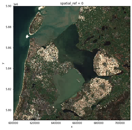
As we can see, the overview image is much smaller compared to the original true color image. Therefore the visualization is much faster. If we are interested in the crop fields, then we would like to know where these are located in the image. To compare its coverage with the raster data, we first check the coordinate systems of both raster and vector data. For raster data, we use pyproj.CRS:

from pyproj import CRS

# Check the coordinate system
CRS(true_color_image.rio.crs)

<Derived Projected CRS: EPSG:32631>
Name: WGS 84 / UTM zone 31N
Axis Info [cartesian]:
- [east]: Easting (metre)
- [north]: Northing (metre)
Area of Use:
- undefined
Coordinate Operation:
- name: UTM zone 31N
- method: Transverse Mercator
Datum: World Geodetic System 1984
- Ellipsoid: WGS 84
- Prime Meridian: Greenwich

To open and check the coordinate system of vector data, we use geopandas:

import geopandas as gpd

# Load the polygons of the crop fields
cf_boundary_crop = gpd.read_file("cropped_field.shp")

# Check the coordinate system
cf_boundary_crop.crs

<Derived Projected CRS: EPSG:28992>
Name: Amersfoort / RD New
Axis Info [cartesian]:
- X[east]: Easting (metre)
- Y[north]: Northing (metre)
Area of Use:
- name: Netherlands - onshore, including Waddenzee, Dutch Wadden Islands and 12-mile offshore coastal zone.
- bounds: (3.2, 50.75, 7.22, 53.7)
Coordinate Operation:
- name: RD New
- method: Oblique Stereographic
Datum: Amersfoort
- Ellipsoid: Bessel 1841
- Prime Meridian: Greenwich

As seen, the coordinate systems differ. To crop the raster using the shapefile, we first convert the coordinate system of cf_boundary_crop to the coordinate system of true_color_image, and then check the coverage:

from matplotlib import pyplot as plt

# Convert the coordinate system
cf_boundary_crop = cf_boundary_crop.to_crs(true_color_image.rio.crs)

# Plot
fig, ax = plt.subplots()
fig.set_size_inches((8,8))

# Plot image
overview_image.plot.imshow(ax=ax)

# Plot crop fields
cf_boundary_crop.plot(
    ax=ax,
    edgecolor="red",
)

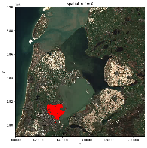
Seeing from the location of the polygons, the crop fields (red) only takes a small part of the raster. Therefore, before actual processing, we can first crop the raster to our area of interest. The clip_box function allows one to crop a raster by the min/max of the x and y coordinates. Note that we are cropping the original image true_color_image now, and not the overview image overview_image.

# Crop the raster with the bounding box
raster_clip_box = true_color_image.rio.clip_box(*cf_boundary_crop.total_bounds)
print(raster_clip_box.shape)

(3, 1565, 1565)

We successfully cropped the raster to a much smaller piece. We can visualize it now:

raster_clip_box.plot.imshow(figsize=(8,8))

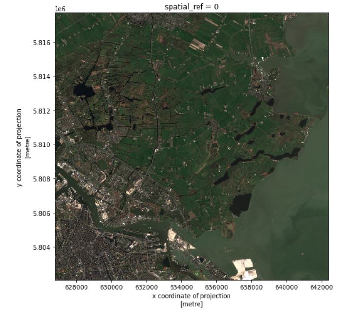
This cropped image can be saved for later usage:

raster_clip_box.rio.to_raster("raster_clip.tif")

Crop raster data with polygons

We have a cropped image around the fields. To further analyze the fields, one may want to crop the image to the exact field boundaries. This can be done with the clip function:

raster_clip_fields = raster_clip_box.rio.clip(cf_boundary_crop['geometry'])

And we can visualize the results:

raster_clip_fields.plot.imshow(figsize=(8,8))

We can save this image for later usage:

raster_clip_fields.rio.to_raster("crop_fields.tif")

Crop raster data with a geometry buffer

It is not always the case that the AoI comes in the format of polygon. Sometimes one would like to perform analysis around a (set of) point(s), or polyline(s). For example, in our AoI, there are also some groundwater monitoring wells available as point vector data. One may also want to perform analysis around these wells. The location of the wells is stored in data/groundwater_monitoring_well.

We can first load the wells vector data, and select wells within the coverage of the image:

# Load wells
wells = gpd.read_file("data/brogmwvolledigeset.zip")
wells = wells.to_crs(raster_clip_box.rio.crs)

# Crop the wells to the image extent
xmin, ymin, xmax, ymax = raster_clip_box.rio.bounds()
wells = wells.cx[xmin:xmax, ymin:ymax]

Then we can check the location of the wells:

# Plot the wells over raster
fig, ax = plt.subplots()
fig.set_size_inches((8,8))
raster_clip_box.plot.imshow(ax=ax)
wells.plot(ax=ax, color='red', markersize=2)

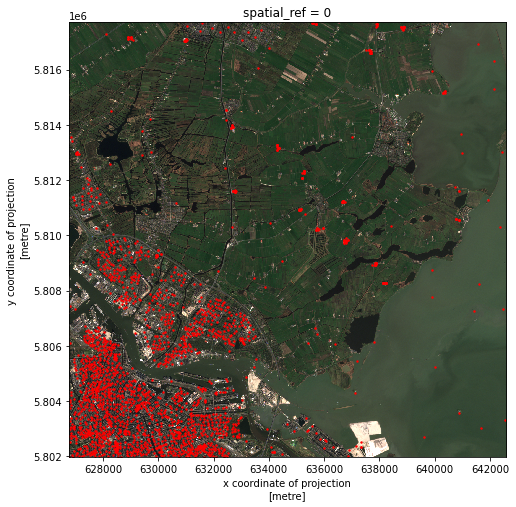
To select pixels around the geometries, one needs to first define a region including the geometries. This region is called a “buffer” and it is defined in the units of the projection. The size of the buffer depends on the analysis in your research. A buffer is also a polygon, which can be used to crop the raster data. geopandas’ objects have a buffer method to generate buffer polygons.

# Create 200m buffer around the wells
wells_buffer = wells.buffer(200)

Now let’s see what do the buffers look like in the image:

# Visualize buffer on raster
fig, ax = plt.subplots()
fig.set_size_inches((8,8))
raster_clip_box.plot.imshow(ax=ax)
wells_buffer.plot(ax=ax, color='red')

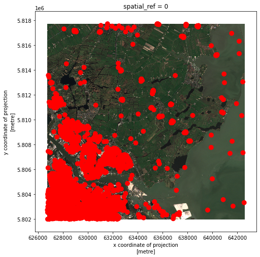
The red dots have grown larger indicating the conversion from points to buffer polygons.

Exercise: Select the raster data around the wells

Now we have the buffer polygons around the groudwater monitoring wells, i.e. wells_buffer. Can you crop the image raster_clip_box to the buffer polygons? Can you visualize the results of cropping?

Solution

# Crop
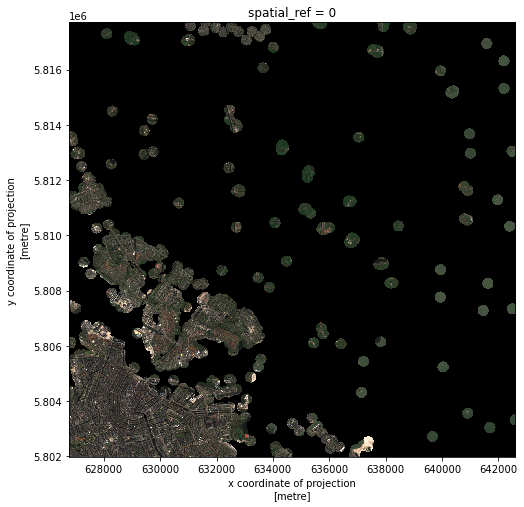
raster_clip_wells = raster_clip_box.rio.clip(wells_buffer)

# Visualize cropped buffer
raster_clip_wells.plot.imshow()

Exercise: Select the raster data around the waterways

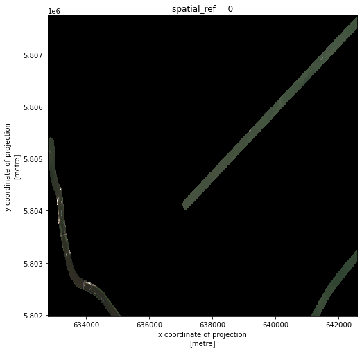
In the previous episode we have corrected the waterway vector data and saved it in waterways_nl_corrected.shp. Can you select out all the raster data within 100m around the waterways, and visualize the results?

Solution

# Load waterways polyline and convert CRS
waterways_nl = gpd.read_file("waterways_nl_corrected.shp")
waterways_nl = waterways_nl.to_crs(raster_clip_box.rio.crs)

# Crop the waterways to the image extent
waterways_nl = waterways_nl.cx[xmin:xmax, ymin:ymax]

# waterways buffer
waterways_nl_buffer = waterways_nl.buffer(100)

# Crop
raster_clip_waterways = raster_clip_box.rio.clip(waterways_nl_buffer)

# Visualize
raster_clip_waterways.plot.imshow(figsize=(8,8))

Crop raster data using another raster dataset

So far we have learned how to crop raster image with vector data. We can also crop a raster with another raster data. In this section, we will demonstrate how to crop the true_color_image image using the crop_fields image.

Using crop_fields raster image

For this section, we will use the crop_fields.tif image that was produced in the section “Crop raster data with polygon”.

We read in the crop_fields.tif image. For the demonstration purpose, we will reproject it to the RD CRS system, so it will be in a different CRS from the true_color_image:

# Read crop_fields
crop_fields = rioxarray.open_rasterio("crop_fields.tif")

# Reproject to RD to make the CRS different from the "true_color_image"
crop_fields = crop_fields.rio.reproject("EPSG:28992")
CRS(crop_fields.rio.crs)

<Derived Projected CRS: EPSG:28992>
Name: Amersfoort / RD New
Axis Info [cartesian]:
- [east]: Easting (metre)
- [north]: Northing (metre)
Area of Use:
- undefined
Coordinate Operation:
- name: unnamed
- method: Oblique Stereographic
Datum: Amersfoort
- Ellipsoid: Bessel 1841
- Prime Meridian: Greenwich

And let’s check again the CRS of true_color_image:

# Get CRS of true_color_image
CRS(true_color_image.rio.crs)

<Derived Projected CRS: EPSG:32631>
Name: WGS 84 / UTM zone 31N
Axis Info [cartesian]:
- [east]: Easting (metre)
- [north]: Northing (metre)
Area of Use:
- undefined
Coordinate Operation:
- name: UTM zone 31N
- method: Transverse Mercator
Datum: World Geodetic System 1984
- Ellipsoid: WGS 84
- Prime Meridian: Greenwich

Now the two images are in different coordinate systems. We can use rioxarray.reproject_match() function to crop true_color_image image. It will perform both the reprojection and the cropping operation. This might take a few minutes, because the true_color_image image is large.

# Crop and reproject
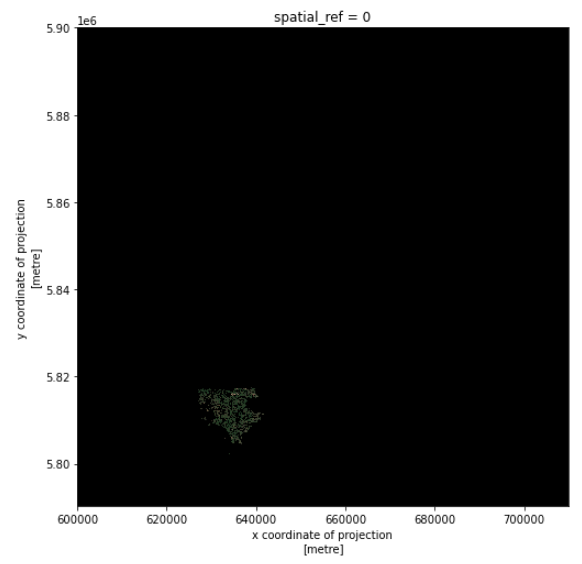
cropped_raster = true_color_image.rio.reproject_match(crop_fields)

# Visualize
cropped_raster.plot.imshow(figsize=(8,8))

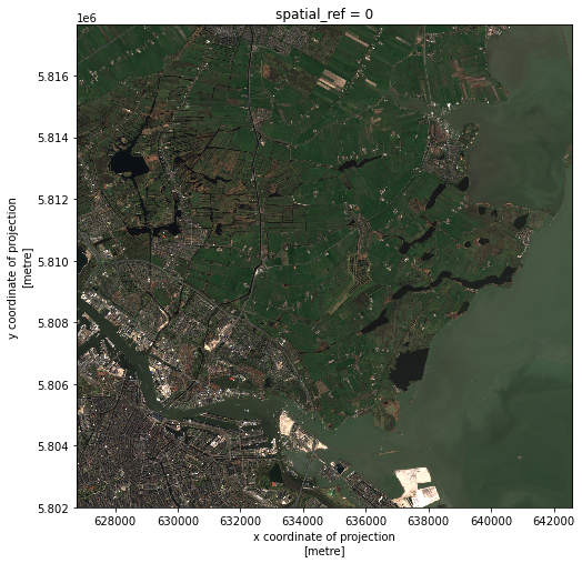
In this way, we accomplish the reproject and cropping in one go.

Exercise

This time let’s do it the other way around by cropping the crop_fields image using the true_color_image image. Discuss the results.

Solution

# Crop
cropped_raster = crop_fields.rio.reproject_match(true_color_image)

# Visualize
cropped_raster.plot.imshow(figsize=(8,8))

In one line reproject_match does a lot of helpful things:

1. It reprojects.
2. It matches the extent using nodata values or by clipping the data.
3. It sets nodata values. This means we can run calculations on those two images.

Code Tip

As we saw before, there also exists a method called reproject(), which only reprojects one raster to another projection. If you want more control over how rasters are resampled, clipped, and/or reprojected, you can use the reproject() method and other rioxarray methods individually.

Key Points

• Use clip_box in DataArray.rio to crop a raster with a bounding box.

• Use clip in DataArray.rio to crop a raster with a given polygon.

• Use buffer in geopandas to make a buffer polygon of a (multi)point or a polyline. This polygon can be used to crop data.

• Use reproject_match function in DataArray.rio to reproject and crop a raster data using another raster data.